General - Globule model - Description of Globule - Construction of Globule system
Based on experience there is no doubt that modeling entire proteins, particularly enzymes, is difficult. First, these systems are large, and the computational effort required for many of the steps involved in modeling can take a long time, often days to weeks. And even when a job ends quite often a minor error is found, particularly in hydrogenation, and the job has to be re-run. Second, given that differences in heats of formation are frequently used in mapping out mechanisms a reliable calculation of the ΔHf is essential. But when entire enzymes are used, quite often minor changes in the active site can result in significant changes far from the active site. This is a consequence of the geometry optimization process - because this process works by minimizing the ΔHf, unavoidable errors in the original placement of hydrogen atoms, particularly those in water molecules, can result in the hydrogen bond lattice being sub-optimal. In principle, errors of this type could be corrected by simulated annealing, but that is also difficult to do.
So in an attempt to simplify modeling of phenomena in enzymes, a new approach has been designed. For convenience this is called a Globule, as in, "Can this simulation be modeled using a Globule?"
A Globule is a model of an active site of an enzyme. This model is large enough to allow docking of ligands and enzyme-catalyzed reaction mechanisms to be explored. At the same time, computational modeling experiments run much faster than if the full enzyme were to be used.
Three important types of calculation can be done in the active region:
(1) Geometry optimization. This is an essential step in all simulations. Setting up and running geometry optimizations is straightforward and reliable, however because these systems are quite large these jobs can take days to run.
(2) Transition state location. Essential for modeling individual steps. Locating and refining transition state geometries is not easy, and even with the Globule model the jobs are very time-consuming, but there are many strategies that can be used. These include following a reaction path, using symmetry when a reaction involves simple bond-breaking - bond-making, and using transition-state location methods, such as LOCATE-TS and SADDLE. Both of these methods use two data-sets, one on each side of the transition state.
(3) Reaction paths. Three types are supported, two of these are the Intrinsic Reaction Coordinate (IRC) and Dynamic Reaction Coordinate (DRC). Both start at the transition state and by moving in one direction along the reaction coordinate, then in the other direction, the reaction path can be mapped out. The third approach is the simple reaction path from stationary point to stationary point. Sometimes following a reaction path can reveal a possible intermediate that had not previously been suggested.
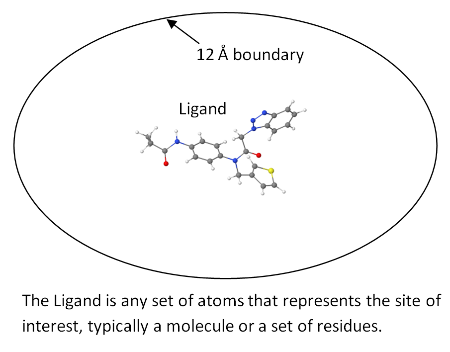
A Globule consists of two parts:
(1) The site of interest. This would normally be defined by the ligand(s) non-covalently bound to the enzyme or a set of residues that take part in a reaction mechanism.
(2) All atoms that are within 12 Ångstroms
of any ligand atom in the site of interest.
The assumption is made that the entire system is available as a normal PDB file. At this point it is not necessary that the system includes hydrogen atoms, in fact if they are present they will be deleted in the first step. All that is needed is a file in PDB format that contains the non-hydrogen atoms of enzyme, the ligand(s) and whatever small molecules, e.g., oxygen atoms of water molecules, are present. For the purposes of this discussion the PDB file will be named 1ABC.pdb, and the ligands will be identified as having residue names and numbers LIA-400 and LIB-401, and have the chain-letter K.
A MOPAC data-set, "Step-1.mop", is constructed. This would have the form:
GEO_DAT="1ABC.pdb" OPT("K 400"=12,"K 401"=12) 0SCF HTML OUTPUT Identify all atoms within 12 Angstroms of residues 400 and 401 |
Keywords HTML and OUTPUT are not really necessary, but they make working with these systems much easier.
When this job is run, it generates an ARC file that has the optimization flags of all atoms within 12 Ångstroms of any atom in either ligand set to "+1" and the optimization flags of all other atoms set to "+0".
Isolating all the atoms to be used, i.e., those with the flags "+1", is not done using MOPAC, instead this task is performed using applications that depend on which operating system is being used. Commands of the type:
|
Windows: |
find "+1" Step-1.arc > Step-2.txt |
| Linux and Mac: |
grep +1 Step-1.arc > Step-2.txt |
would likely be useful here. This operation is called Step 2, so for convenience the file-name Step-2.mop is not used, instead the data-set in the next step, which does use MOPAC, will be referred to as Step-3.mop.
Look at Step-2.txt and delete any lines that are bland or are clearly not atoms, i.e., are not PDB lines. At this point, the system does not look sensible. Some atoms selected by OPT might be isolated from the rest of the system, some groups, such as phenyl rings, might have one or more atoms missing, and some residues might be incomplete.
There are two options for selecting the atoms that are to be included in the globule.
Option 1: Inspect the system, and delete all moieties at the surface of the globule that are not covalently bound to the protein. This includes fragments of residues and water oxygen atoms that would be near the boundary. These entities should be deleted because if they were not they would be converted into small molecules in the next step, and later on they might drift to form non-covalent bonds with the rest of the globule.
Option 2: Inspect the system, and identify all the residues present in the globule. Edit either the original file 1ABC.pdb or the ARC file Step-1.arc to include all atoms in every residue in the globule. Also include the water oxygen atoms that are inside the globule but not near to the boundary. Flag all atoms for optimization. Name the resulting file "Step-2.txt"
Hydrogenation is done in two steps. First, all atoms that can be hydrogenated are hydrogenated. This gives rise to a system in which everything that can be neutral is in fact neutral, that is at this point there are no ionized residues or molecules. The only atoms that would be ionized at this point are those that are always ionized, such as the alkali metal atoms.
A data-set named "Step-3.mop" for this would have the following form:
HTML ADD-H GEO_DAT="Step-2.txt" OUTPUT Simple hydrogenation of system in Step-2 - this gives the template hydrogenation for Step-4 to modify |
As expected, this operation hydrogenates all the residues and ligands and other small molecules.
It also hydrogenates atoms that might have "dangling valencies" - atoms that were near to the 12 �ngstrom boundary and one or more atoms that were bonded to
them were outside the boundary and therefore excluded from the system. If any fragments described in step 2 were not deleted, these would give rise to some strange compounds such as ammonia, methane, formaldehyde, etc. Although compounds of this type are normally not important and could be ignored, to prevent the possibility of these small molecules from drifting and possibly forming hydrogen bonds with the protein, thus changing the heat of formation of the system, it is important to delete all moieties of this type at this point.
The default hydrogenation is almost never correct. Each system has its own identifiable set of ionized sites, and individual hydrogen atoms should be added and deleted so as to achieve the correct ionization. In addition, sometimes a PDB file has a severe geometric error that causes the bond-order between two atoms to be wrongly assigned. This kind of error must also be corrected by selectively adding or deleting hydrogen atoms. Over the past decade the number of errors of this type in PDB files has dropped significantly, but for older PDB files there is a real possibility of encountering errors of this type.
Adjusting the hydrogenation is best done iteratively. To begin with, a list of the sites that should be ionized must be constructed. Then using a data-set named "Step-4a.mop" of the type:
HTML GEO_DAT="Step-3.arc" OUTPUT SITE=(text) Adjust the hydrogenation from Step-3 to produce the starting geometry for optimizations |
add and delete hydrogen atoms using the keyword SITE to achieve the desired effect. Each change is specified by an entry in "text" so, for example, if an oxygen atom on a phosphate group needed to be ionized, the keyword could be SITE=("[PO4]401:A.O2"(-))
Run Step-4a.mop. This run does not generate a list of ionized sites, so make a second data-set named "Step-4b.mop" that has the following keywords:
HTML GEO_DAT="Step-4a.arc" OUTPUT CHARGES Identify all charged sites |
Run Step-4b.mop and look at the list of charged sites in the output. Also look at the geometry using a GUI. Check that the hydrogenation and ionization are correct. If there are any faults, edit Step-4.mop to correct them, and re-run Step-4a.mop and Step-4b.mop.
Only after the hydrogenation is correct should the move to Step 5 be made.
This job, "Step-5.mop", requires a significant amount of CPU time, so specify a long time, three weeks are allowed in the example below. In practice, the job will run in a much smaller time so this option simply means that it won't run out of time. From here on all jobs will need MOZYME. An important safety feature is to always use keyword CHARGE. If, as often happens in complicated reactions, the Lewis structure changes so that the computed net charge also changes resulting in the computed charge changing, the presence of this keyword would result in the user being alerted, then corrective action, typically using CVB or SETPI, can be taken to ensure that the net charge is reset to its original value.
MOZYME CHARGE=n HTML T=3W GEO_DAT="Step-5.arc" EPS=78.4 LET(100) 1SCF Starting geometry, with positions of all atoms optimized |
Before running this job check for errors. Compare the list of charged sites in the output file with the list of sites that should be ionized that was constructed for Step 4. Investigate any differences and take the appropriate action.
Run this job then look at the output to verify that everything is okay.
When everything looks good, replace the keyword 1SCF with OUTPUT, then run the job. it will likely take several days to run. Sometimes salt bridges form spontaneously, if that occurs and the salt bridge looks correct then no action needs to be taken.
The result of the Step-5 job will be a good starting geometry for further work. It's important to carefully save this geometry so that it can be used as the starting point for other jobs. To do this, proceed as follows:
Create a new folder named "Starting model", and move into it. Copy the ARC file from Step-5 into this new folder. Give this file a descriptive name, e.g. "Reactants 1SCF.mop". Edit the data-set to run a single SCF calculation, e.g.:
MOZYME CHARGE=n HTML 1SCF GEO_DAT="Step-5.arc" GRADIENTS OUTPUT Starting model, one SCF |
then run that job. Do not delete any of the files generated in this process because they are useful reference files for documenting the work and the ARC file will be useful in constructing other datasets. If an error is found in this job, locate the cause in "Preparing Starting Model", correct it, and copy the corrected ARC file into "Starting model" and re-run the job there. This somewhat lengthy procedure is designed to ensure that folders containing important results do not get damaged by user-errors.